Example FlowSOM Pipeline

This vignette describes a protocol for analyzing high-dimensional cytometry data using FlowSOM, a clustering and visualization algorithm based on a self-organizing map (SOM). FlowSOM is used to distinguish cell populations from cytometry data in an unsupervised way and can help to gain deeper insights in fields such as immunology and oncology.

Loading in the data

FlowSOM handles different inputs, such as an anndata object by pytometry or a filepath. For this purpose we will make use of an anndata object. This allows easier preprocessing. Note that this requires also installing the pytometry package (version > 0.1.5) with e.g. pip install pytometry.

# Import modules
import flowsom as fs
import pytometry as pm
import scanpy as sc
import csv
import numpy as np
import matplotlib.pyplot as plt

# set default plotting parameters
plt.rcParams["figure.figsize"] = (6.5, 4.8)
plt.rcParams["figure.dpi"] = 300
plt.rcParams["font.size"] = 10

# Load data
ff = fs.io.read_FCS("../../tests/data/not_preprocessed.fcs")
ff

AnnData object with n_obs × n_vars = 19225 × 18
    var: 'n', 'channel', 'marker', '$PnB', '$PnE', '$PnG', '$PnR', '$PnV'
    uns: 'meta'

We can get an overview of the most important data in our anndata object by using var. All the metadata is stored in a dictionary at ff.uns["meta]

ff.var

	n	channel	marker	$PnB	$PnE	$PnG	$PnR	$PnV
Time	1	Time		32	0,0	0.01	262144
FSC-A	2	FSC-A		32	0,0	1.0	262144	280
FSC-H	3	FSC-H		32	0,0	1.0	262144	280
FSC-W	4	FSC-W		32	0,0	1.0	262144	280
SSC-A	5	SSC-A		32	0,0	1.0	262144	280
SSC-H	6	SSC-H		32	0,0	1.0	262144	280
SSC-W	7	SSC-W		32	0,0	1.0	262144	280
GFP	8	FITC-A	GFP	32	0,0	1.0	262144	412
CD8	9	Pacific Blue-A	CD8	32	0,0	1.0	262144	417
l/d	10	AmCyan-A	l/d	32	0,0	1.0	262144	496
Qdot 605-A	11	Qdot 605-A		32	0,0	1.0	262144	588
TCRyd	12	APC-A	TCRyd	32	0,0	1.0	262144	597
CD45	13	Alexa Fluor 700-A	CD45	32	0,0	1.0	262144	492
TCRb	14	APC-Cy7-A	TCRb	32	0,0	1.0	262144	511
NK1/1	15	PE-A	NK1/1	32	0,0	1.0	262144	505
CD4	16	PE-Texas Red-A	CD4	32	0,0	1.0	262144	560
CD19	17	PE-Cy5-A	CD19	32	0,0	1.0	262144	593
CD3	18	PE-Cy7-A	CD3	32	0,0	1.0	262144	588

ff.uns["meta"].keys()

dict_keys(['__header__', '$BEGINANALYSIS', '$BEGINDATA', '$BEGINSTEXT', '$BTIM', '$BYTEORD', '$DATATYPE', '$DATE', '$ENDANALYSIS', '$ENDDATA', '$ENDSTEXT', '$ETIM', '$FIL', '$INST', '$MODE', '$NEXTDATA', '$PAR', '$SRC', '$SYS', '$TIMESTEP', '$TOT', 'APPLY COMPENSATION', 'AUTOBS', 'CREATOR', 'EXPERIMENT NAME', 'EXPORT TIME', 'EXPORT USER NAME', 'FCSversion', 'FILENAME', 'flowCore_$P10Rmax', 'flowCore_$P10Rmin', 'flowCore_$P11Rmax', 'flowCore_$P11Rmin', 'flowCore_$P12Rmax', 'flowCore_$P12Rmin', 'flowCore_$P13Rmax', 'flowCore_$P13Rmin', 'flowCore_$P14Rmax', 'flowCore_$P14Rmin', 'flowCore_$P15Rmax', 'flowCore_$P15Rmin', 'flowCore_$P16Rmax', 'flowCore_$P16Rmin', 'flowCore_$P17Rmax', 'flowCore_$P17Rmin', 'flowCore_$P18Rmax', 'flowCore_$P18Rmin', 'flowCore_$P1Rmax', 'flowCore_$P1Rmin', 'flowCore_$P2Rmax', 'flowCore_$P2Rmin', 'flowCore_$P3Rmax', 'flowCore_$P3Rmin', 'flowCore_$P4Rmax', 'flowCore_$P4Rmin', 'flowCore_$P5Rmax', 'flowCore_$P5Rmin', 'flowCore_$P6Rmax', 'flowCore_$P6Rmin', 'flowCore_$P7Rmax', 'flowCore_$P7Rmin', 'flowCore_$P8Rmax', 'flowCore_$P8Rmin', 'flowCore_$P9Rmax', 'flowCore_$P9Rmin', 'FSC ASF', 'GUID', 'ORIGINALGUID', 'P10BS', 'P10DISPLAY', 'P10MS', 'P11BS', 'P11DISPLAY', 'P11MS', 'P12BS', 'P12DISPLAY', 'P12MS', 'P13BS', 'P13DISPLAY', 'P13MS', 'P14BS', 'P14DISPLAY', 'P14MS', 'P15BS', 'P15DISPLAY', 'P15MS', 'P16BS', 'P16DISPLAY', 'P16MS', 'P17BS', 'P17DISPLAY', 'P17MS', 'P18BS', 'P18DISPLAY', 'P18MS', 'P1BS', 'P1MS', 'P2BS', 'P2DISPLAY', 'P2MS', 'P3BS', 'P3DISPLAY', 'P3MS', 'P4BS', 'P4MS', 'P5BS', 'P5DISPLAY', 'P5MS', 'P6BS', 'P6DISPLAY', 'P6MS', 'P7BS', 'P7MS', 'P8BS', 'P8DISPLAY', 'P8MS', 'P9BS', 'P9DISPLAY', 'P9MS', 'THRESHOLD', 'transformation', 'TUBE NAME', 'WINDOW EXTENSION', 'channels', 'header', 'spill'])

Additionaly we can read in a csv file as well.

ff_csv = fs.io.read_csv("../../tests/data/fcs.csv")
ff_csv

AnnData object with n_obs × n_vars = 19225 × 18
    var: 'n', 'channel', 'marker'

The FlowSOM function accepts an anndata object or a filepath to a fcs or csv file. The FlowSOM function will return a FlowSOM mudata object. This object contains all the information about the SOM and the clustering.

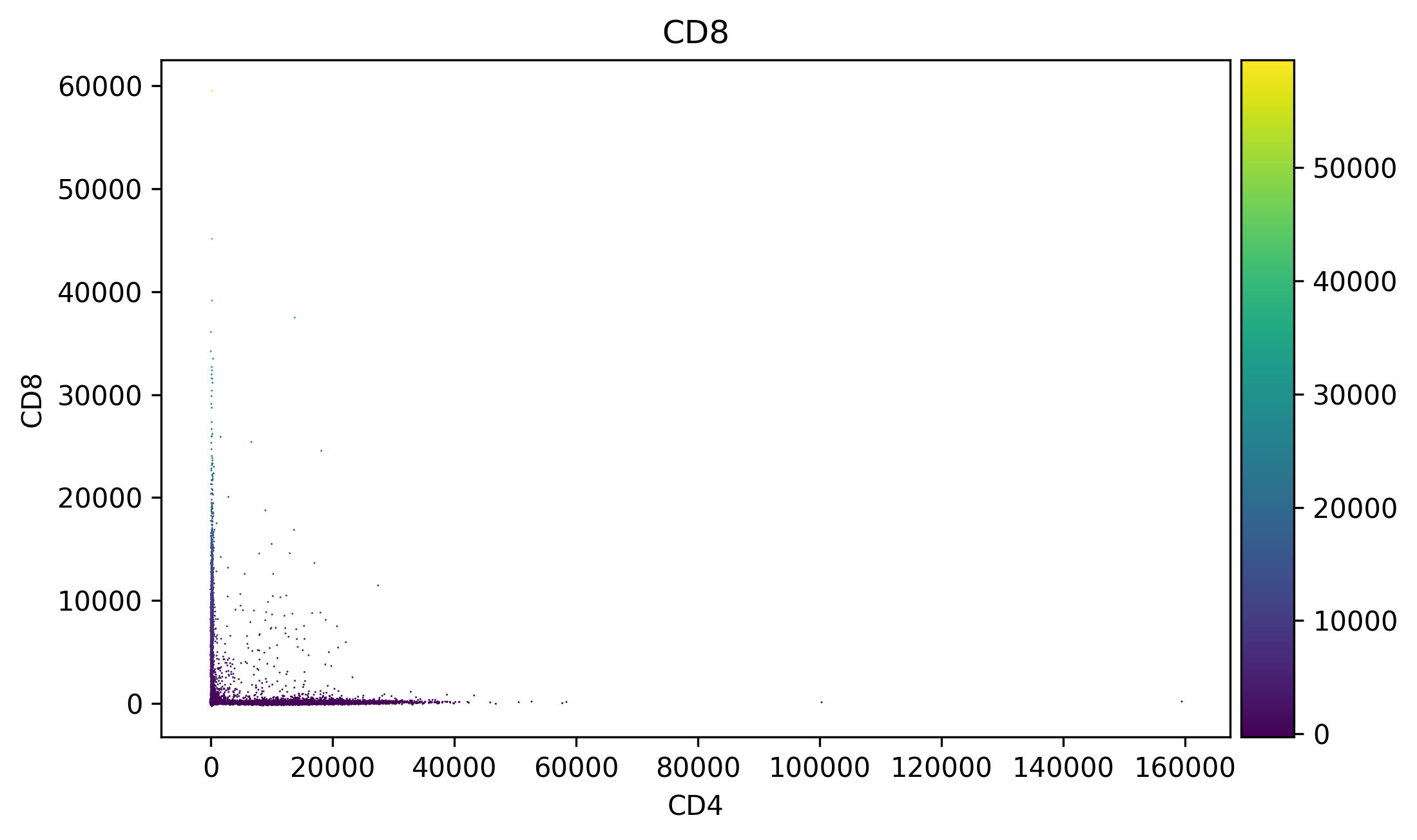
# Visualize data
sc.pl.scatter(ff, x="CD4", y="CD8", color="CD8", size=2)

Preprocessing

We start with compensating the data and then we transform the data with the logicle function. For CyTOF data an arcsinh transformation is preferred which is also found in the pytometry package. Besides compensation and transformation, we also recommend cleaning the data by removing margin events and by using cleaning algorithms.

# Compensate
ff_comp = pm.pp.compensate(ff, inplace=False)

cols_to_use = [8, 11, 13, 14, 15, 16, 17]
colnames_to_use = ff_comp[:, cols_to_use].var_names.tolist()
colnames_to_use

['CD8', 'TCRyd', 'TCRb', 'NK1/1', 'CD4', 'CD19', 'CD3']

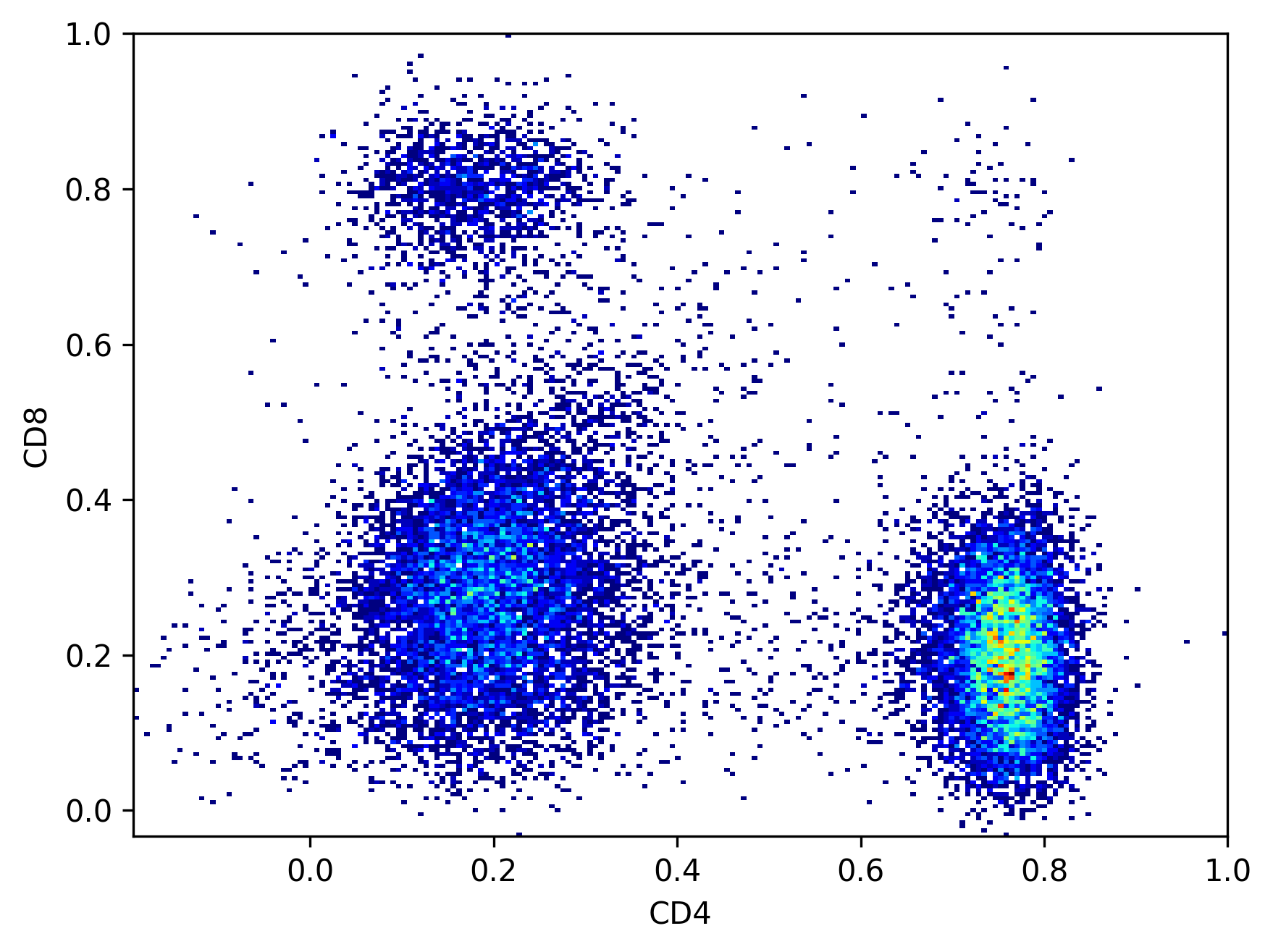
# Transform
ff_t = pm.tl.normalize_autologicle(ff_comp, channels=colnames_to_use, inplace=False)

# Visualize data
ax = plt.hist2d(ff_t[:, "CD4"].X.flatten(), ff_t[:, "CD8"].X.flatten(), bins=200, cmin=1, cmap="jet")
plt.xlabel("CD4")
plt.ylabel("CD8")
plt.show()

FlowSOM

The easiest way to use this package is using the wrapper function FlowSOM, although it has less options than using the underlying functions separately. It holds the data in a MuData object, of which the first modality is the cell data and the second modality is the cluster data. We will cluster the data with a 10 x 10 SOM grid and 10 metaclusters. Notice that due to the just-in-time compilation of numba, the first run of FlowSOM can take a while and the subsequent runs will be much faster. We also set the seed here to make sure the analysis is deterministic and reproducible.

fsom = fs.FlowSOM(ff_t.copy(), cols_to_use=cols_to_use, n_clusters=10, xdim=10, ydim=10, seed=42)

We can inspect the underlying model and can see it’s like any other scikit-learn model. The FlowSOM estimator first overclusters using a cluster_model (Self-Organizing Map). Then it uses a metacluster_model (Consensus Agglomerative Clustering) to merge the clusters into metaclusters.

fsom.model

FlowSOMEstimator(cluster_model=SOMEstimator(codes=array([[ 0.19228934,  0.1865745 ,  0.23266686,  0.87238413,  0.05209107,
         0.3103338 ,  0.21093693],
       [ 0.37591392,  0.26387554,  0.21212712,  0.5848203 ,  0.21481907,
         0.26141116,  0.21131037],
       [ 0.428116  ,  0.27063912,  0.32987905,  0.46879607,  0.3014614 ,
         0.24979484,  0.21359852],
       [ 0.71539164,  0.25424176,  0.22920464,  0.38272676,  0.49828213,
         0.2463...
       [ 0.16985969,  0.12226646,  0.56166893,  0.25476876,  0.7380235 ,
         0.40652   ,  0.7086935 ],
       [ 0.27684072,  0.16656815,  0.6013744 ,  0.11409374,  0.7604119 ,
         0.36639097,  0.735394  ],
       [ 0.1659379 ,  0.27120367,  0.5247936 ,  0.12309174,  0.7345894 ,
         0.2421986 ,  0.67283285],
       [ 0.2248714 ,  0.31179267,  0.61458   ,  0.05833715,  0.773493  ,
         0.13654871,  0.74112475]], dtype=float32),
                                            seed=42),
                 metacluster_model=ConsensusCluster(K=10, n_clusters=10))

In a Jupyter environment, please rerun this cell to show the HTML representation or trust the notebook.
On GitHub, the HTML representation is unable to render, please try loading this page with nbviewer.org.

The output is stored in a MuData object, containing two AnnData object: cell_data (n_cells x n_features) and cluster_data (n_SOM_nodes x n_features).

fsom.mudata

MuData object with n_obs × n_vars = 0 × 0
  2 modalities
    cell_data:	19225 x 18
      obs:	'clustering', 'distance_to_bmu', 'metaclustering'
      var:	'n', 'channel', 'marker', '$PnB', '$PnE', '$PnG', '$PnR', '$PnV', 'pretty_colnames', 'markers', 'channels', 'cols_used'
      uns:	'meta', 'n_nodes', 'n_metaclusters'
      layers:	'original'
    cluster_data:	100 x 18
      obs:	'percentages', 'metaclustering'
      uns:	'xdim', 'ydim', 'outliers', 'metacluster_MFIs', 'graph'
      obsm:	'cv_values', 'sd_values', 'mad_values', 'codes', 'grid', 'layout'

We can access the cell data and the cluster data with the get_cell_data() and get_cluster_data() functions.

The cell data is an anndata object that contains the original cell data. As observations, we find the clustering, metaclustering and distance to best matching unit per cell. In var, we find the pretty colnames, i.e. a combination of markers and channels, the markers, the channels and a boolean mask of the columns used for clustering. n_nodes and n_metaclusters in uns contain the number of clusters and metaclusters respectively.

fsom.get_cell_data()

AnnData object with n_obs × n_vars = 19225 × 18
    obs: 'clustering', 'distance_to_bmu', 'metaclustering'
    var: 'n', 'channel', 'marker', '$PnB', '$PnE', '$PnG', '$PnR', '$PnV', 'pretty_colnames', 'markers', 'channels', 'cols_used'
    uns: 'meta', 'n_nodes', 'n_metaclusters'
    layers: 'original'

The cluster data contains the original median values per cluster per marker. In obsm, we find the cv values, sd values, mad values, coordinates of the nodes, coordinates of the the grid and the coordinates of the MST layout. The xdim, ydim, outliers, igraph object and metacluster MFIs can be found in uns.

fsom.get_cluster_data()

AnnData object with n_obs × n_vars = 100 × 18
    obs: 'percentages', 'metaclustering'
    uns: 'xdim', 'ydim', 'outliers', 'metacluster_MFIs', 'graph'
    obsm: 'cv_values', 'sd_values', 'mad_values', 'codes', 'grid', 'layout'

fsom.get_cell_data().var

	n	channel	marker	$PnB	$PnE	$PnG	$PnR	$PnV	pretty_colnames	markers	channels	cols_used
Time	1	Time		32	0,0	0.01	262144		Time <Time>	Time	Time	False
FSC-A	2	FSC-A		32	0,0	1.0	262144	280	FSC-A <FSC-A>	FSC-A	FSC-A	False
FSC-H	3	FSC-H		32	0,0	1.0	262144	280	FSC-H <FSC-H>	FSC-H	FSC-H	False
FSC-W	4	FSC-W		32	0,0	1.0	262144	280	FSC-W <FSC-W>	FSC-W	FSC-W	False
SSC-A	5	SSC-A		32	0,0	1.0	262144	280	SSC-A <SSC-A>	SSC-A	SSC-A	False
SSC-H	6	SSC-H		32	0,0	1.0	262144	280	SSC-H <SSC-H>	SSC-H	SSC-H	False
SSC-W	7	SSC-W		32	0,0	1.0	262144	280	SSC-W <SSC-W>	SSC-W	SSC-W	False
FITC-A	8	FITC-A	GFP	32	0,0	1.0	262144	412	GFP <FITC-A>	GFP	FITC-A	False
Pacific Blue-A	9	Pacific Blue-A	CD8	32	0,0	1.0	262144	417	CD8 <Pacific Blue-A>	CD8	Pacific Blue-A	True
AmCyan-A	10	AmCyan-A	l/d	32	0,0	1.0	262144	496	l/d <AmCyan-A>	l/d	AmCyan-A	False
Qdot 605-A	11	Qdot 605-A		32	0,0	1.0	262144	588	Qdot 605-A <Qdot 605-A>	Qdot 605-A	Qdot 605-A	False
APC-A	12	APC-A	TCRyd	32	0,0	1.0	262144	597	TCRyd <APC-A>	TCRyd	APC-A	True
Alexa Fluor 700-A	13	Alexa Fluor 700-A	CD45	32	0,0	1.0	262144	492	CD45 <Alexa Fluor 700-A>	CD45	Alexa Fluor 700-A	False
APC-Cy7-A	14	APC-Cy7-A	TCRb	32	0,0	1.0	262144	511	TCRb <APC-Cy7-A>	TCRb	APC-Cy7-A	True
PE-A	15	PE-A	NK1/1	32	0,0	1.0	262144	505	NK1/1 <PE-A>	NK1/1	PE-A	True
PE-Texas Red-A	16	PE-Texas Red-A	CD4	32	0,0	1.0	262144	560	CD4 <PE-Texas Red-A>	CD4	PE-Texas Red-A	True
PE-Cy5-A	17	PE-Cy5-A	CD19	32	0,0	1.0	262144	593	CD19 <PE-Cy5-A>	CD19	PE-Cy5-A	True
PE-Cy7-A	18	PE-Cy7-A	CD3	32	0,0	1.0	262144	588	CD3 <PE-Cy7-A>	CD3	PE-Cy7-A	True

flowsom_clustering

Alternatively to working with this FlowSOM object, we can simply add the FlowSOM clustering and metaclustering to an existing AnnData object. The convenience function flowsom_clustering is available and is similar to other clustering methods in the scverse. The FlowSOM clustering and metaclustering can be found in .obs and the parameters used in the FlowSOM clustering in .uns.FlowSOM.

ff_clustered = fs.flowsom_clustering(ff_t, cols_to_use, xdim=10, ydim=10, n_clusters=10, seed=42)
ff_clustered

AnnData object with n_obs × n_vars = 19225 × 18
    obs: 'FlowSOM_clusters', 'FlowSOM_metaclusters'
    var: 'n', 'channel', 'marker', '$PnB', '$PnE', '$PnG', '$PnR', '$PnV'
    uns: 'meta', 'FlowSOM'
    layers: 'original'

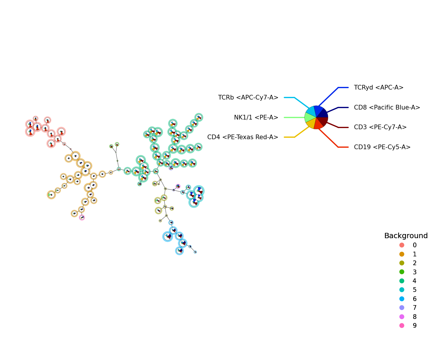
FlowSOM visualizations

A FlowSOM object can be visualized with the plot_stars() function

p = fs.pl.plot_stars(fsom, background_values=fsom.get_cluster_data().obs.metaclustering)

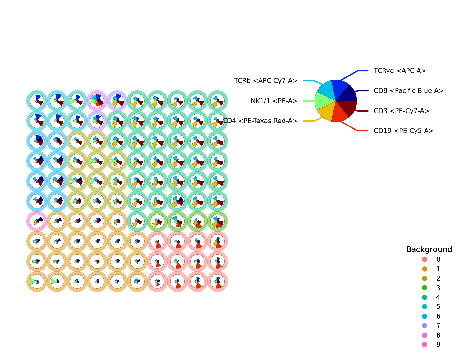
We can also visualize the grid, to reduce overlap and get a better view of the data. The node sizes of the nodes and/or the background nodes can be made equal with the equal_node_size or equal_background_size argument

p = fs.pl.plot_stars(
    fsom,
    background_values=fsom.get_cluster_data().obs.metaclustering,
    view="grid",
    equal_node_size=True,
    equal_background_size=True,
)

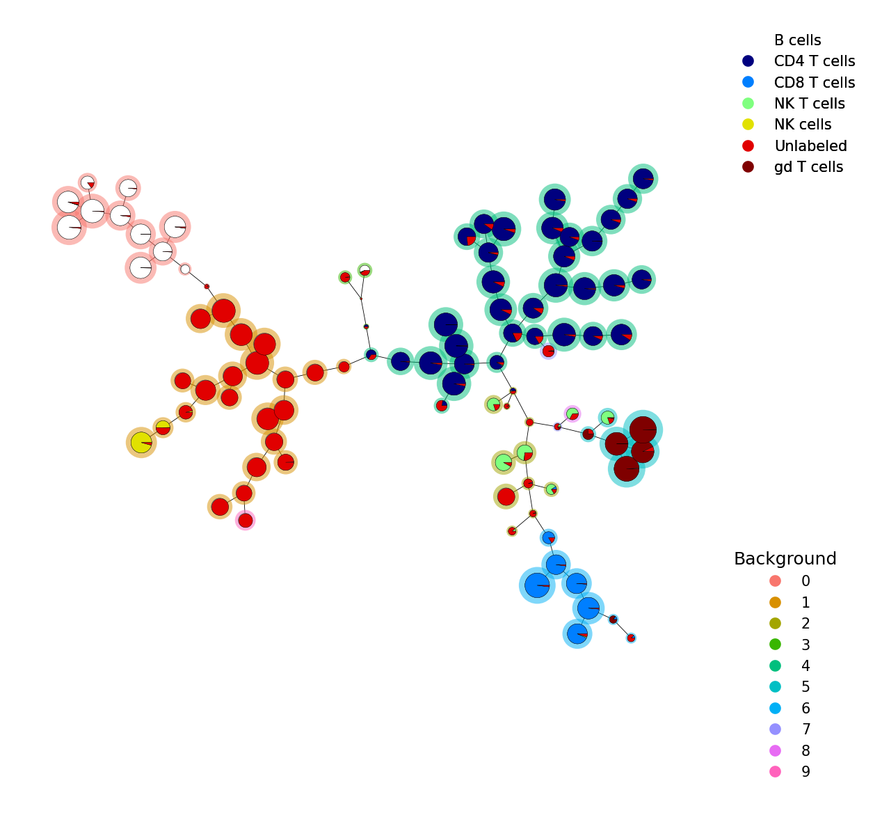
If you have a label for every cell, we can visualize this with plot_pies(). Here every node is a piechart with the percentage of cells in each cluster.

# Read in that data
file = open("../../tests/data/gating_result.csv")
data = csv.reader(file)
data = [i[0] for i in data]

# Plot
p = fs.pl.plot_pies(fsom, data, background_values=fsom.get_cluster_data().obs.metaclustering)

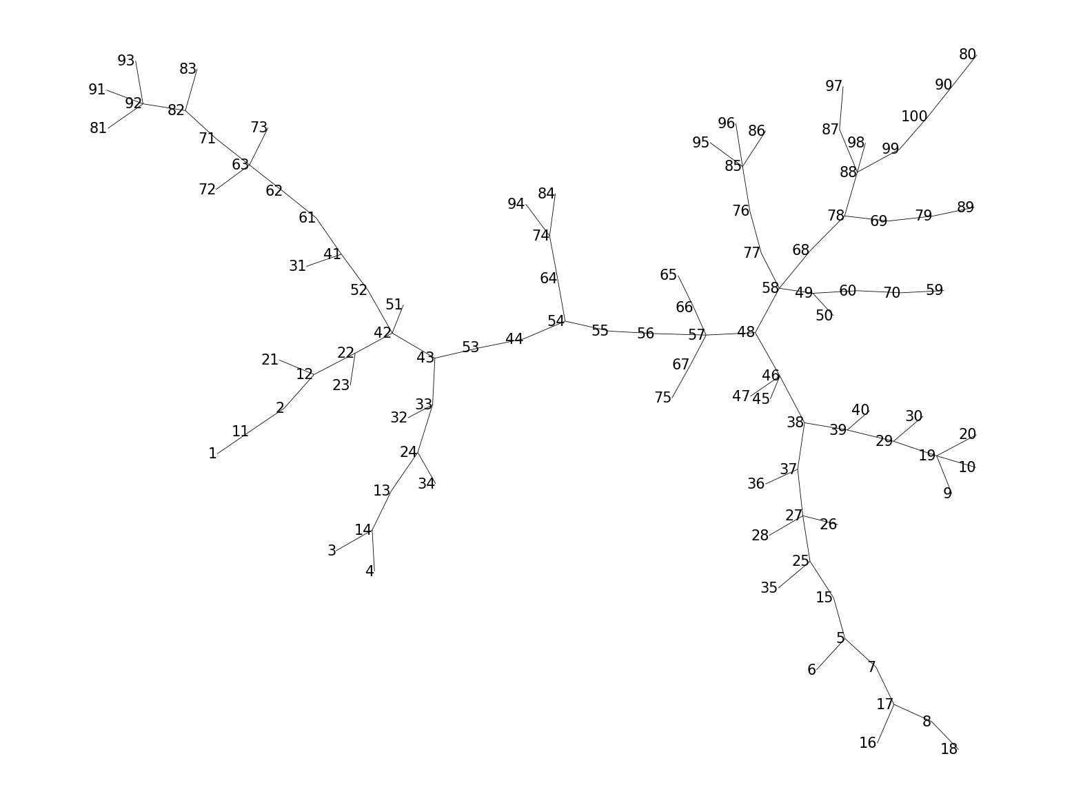
We can also visualize the cluster numbers or metacluster numbers with the help of plot_numbers(), if level="clusters" or level="metaclusters", respectively. This functions uses plot_labels() internally, to which one can pass custom labels, such as the cell type labels.

p = fs.pl.plot_numbers(fsom, level="clusters", text_size=5)

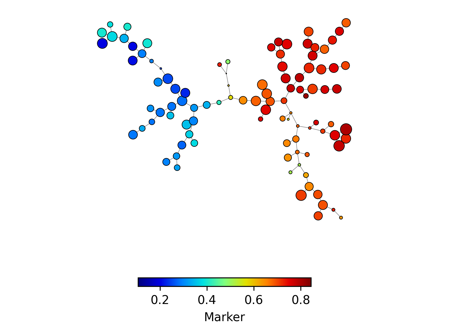
It is possible to visualize one marker on a FlowSOM tree with the plot_marker() function. This function uses the plot_variable() function internally, to which one can pass custom variables, such as the cell type labels.

p = fs.pl.plot_marker(fsom, marker=np.array(["CD3"]))

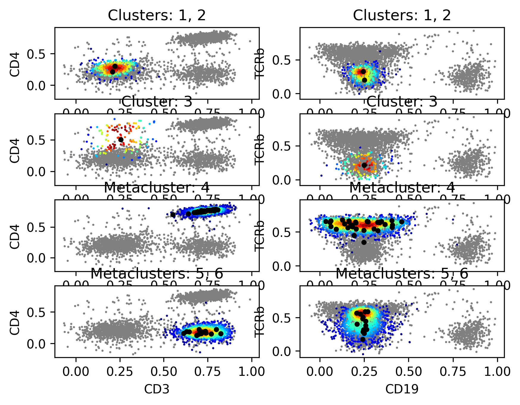
We can also visualize the clusters and metaclusters on a 2D scatter plot with plot_2D_scatters().

p = fs.pl.plot_2D_scatters(
    fsom,
    channelpairs=[["CD3", "CD4"], ["CD19", "TCRb"]],
    clusters=[[1, 2], [3]],
    metaclusters=[[4], [5, 6]],
    density=True,
    centers=True,
)

Downstream analysis

We might need the percentages, counts or the percentages of positive cells per cluster or metacluster and per file for further analysis. This can be done with the get_features() function. This function returns a dictionary containing pandas of the requested data.

features = fs.tl.get_features(
    fsom,
    files=[ff_t[1:1000, :], ff_t[1000:2000, :]],
    level=["clusters", "metaclusters"],
    type=["counts", "percentages"],
)
features["metacluster_percentages"]

	MC0	MC1	MC2	MC3	MC4	MC5	MC6	MC7	MC8	MC9
0	0.134134	0.253253	0.038038	0.007007	0.38038	0.088088	0.087087	0.009009	0.002002	0.001001
1	0.133000	0.227000	0.038000	0.003000	0.40100	0.090000	0.099000	0.001000	0.004000	0.004000

The counts, percentages, percentages_positive, per cluster or metacluser can also extracted from a FlowSOM object. For this we can use get_counts(), get_percentages(), get_cluster_percentages_positive() or get_metacluster_percentages_positive, respectively.

fs.tl.get_counts(fsom, level="clusters")

	counts
C0	258
C1	110
C2	171
C3	114
C4	230
...	...
C95	222
C96	271
C97	219
C98	245
C99	231

100 rows × 1 columns

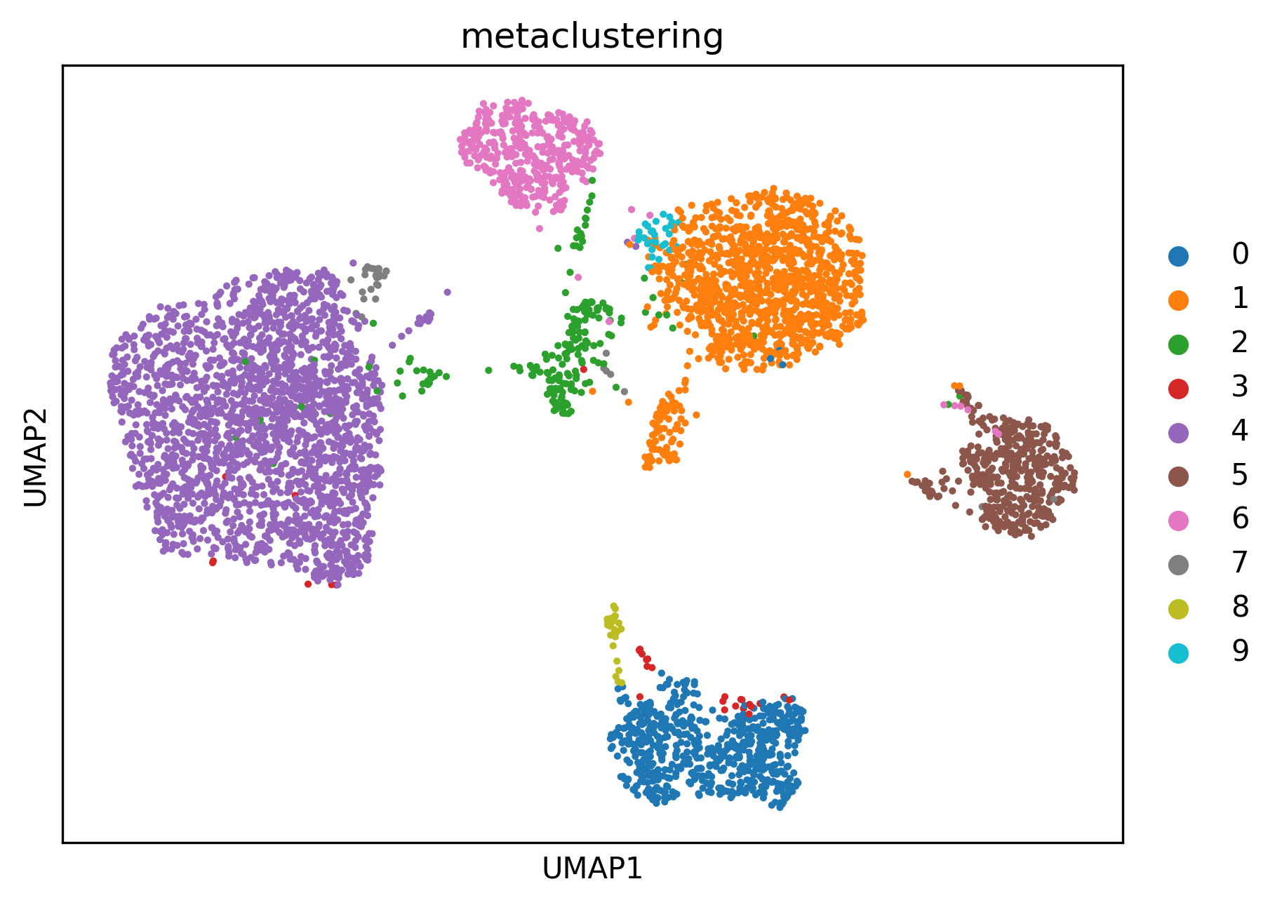
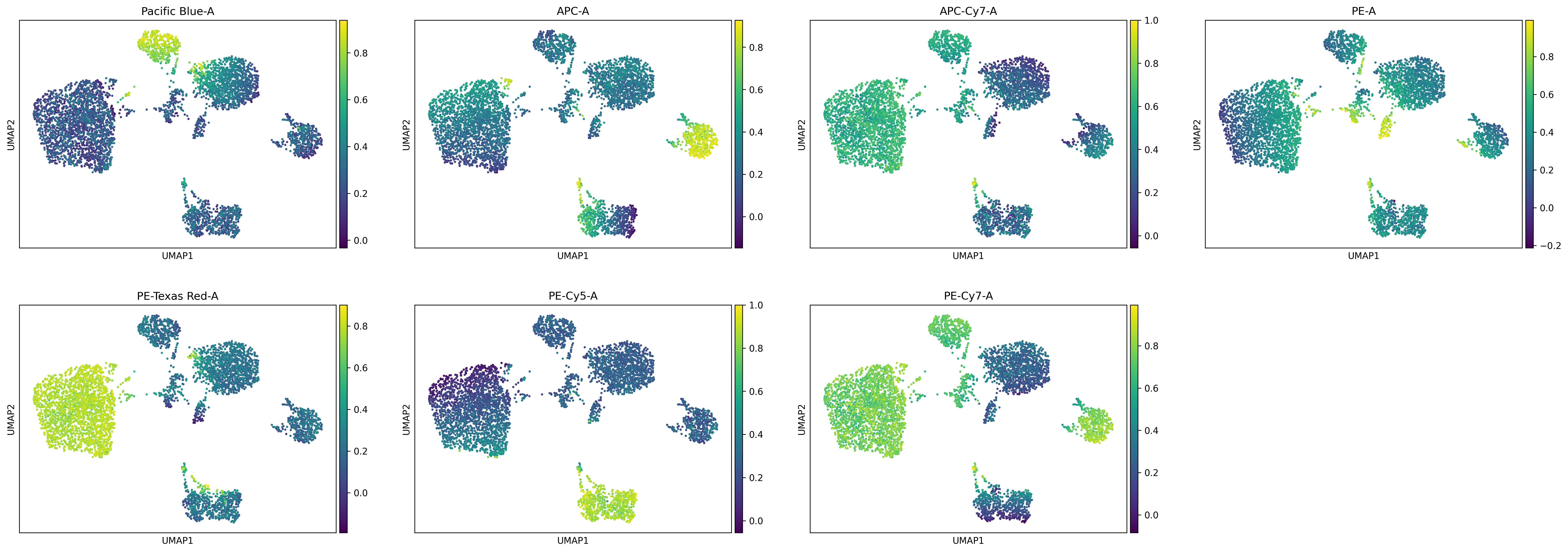
At last it is also possible to visualize a UMAP colored by the metaclustering or the expression of a marker. For this we will use scanpy.

# Get subset of the cell data
ref_markers_bool = fsom.get_cell_data().var["cols_used"]
subset_fsom = fsom.get_cell_data()[
    np.random.choice(range(fsom.get_cell_data().shape[0]), 5000, replace=False),
    fsom.get_cell_data().var_names[ref_markers_bool],
]
sc.pp.neighbors(subset_fsom)
sc.tl.umap(subset_fsom)

# By metaclustering
subset_fsom.obs["metaclustering"] = subset_fsom.obs["metaclustering"].astype(str)
sc.pl.umap(subset_fsom, color="metaclustering")

# By markers
sc.pl.umap(subset_fsom, color=fsom.get_cell_data().var_names[ref_markers_bool])

Other interesting functions

To get the markers or channels from the corresponding channels or markers of an FCS or a FlowSOM object, we can use get_markers() or get_channels().

newdata subset

fs.tl.get_channels(ff_t, np.array(["CD3", "CD4"]))

{'PE-Cy7-A': 'CD3', 'PE-Texas Red-A': 'CD4'}

fs.tl.get_markers(fsom, np.array(["PE-A", "PE-Cy7-A"]))

{'NK1/1': 'PE-A', 'CD3': 'PE-Cy7-A'}

We can also merge multiple FCS files with random subsampling with the function aggregate_flowframes().

fs.pp.aggregate_flowframes(
    filenames=[
        "../../tests/data/not_preprocessed.fcs",
        "../../tests/data/not_preprocessed.fcs",
    ],
    c_total=5000,
)

AnnData object with n_obs × n_vars = 5000 × 18
    obs: 'Original_ID', 'File', 'File_scattered'
    uns: 'meta'

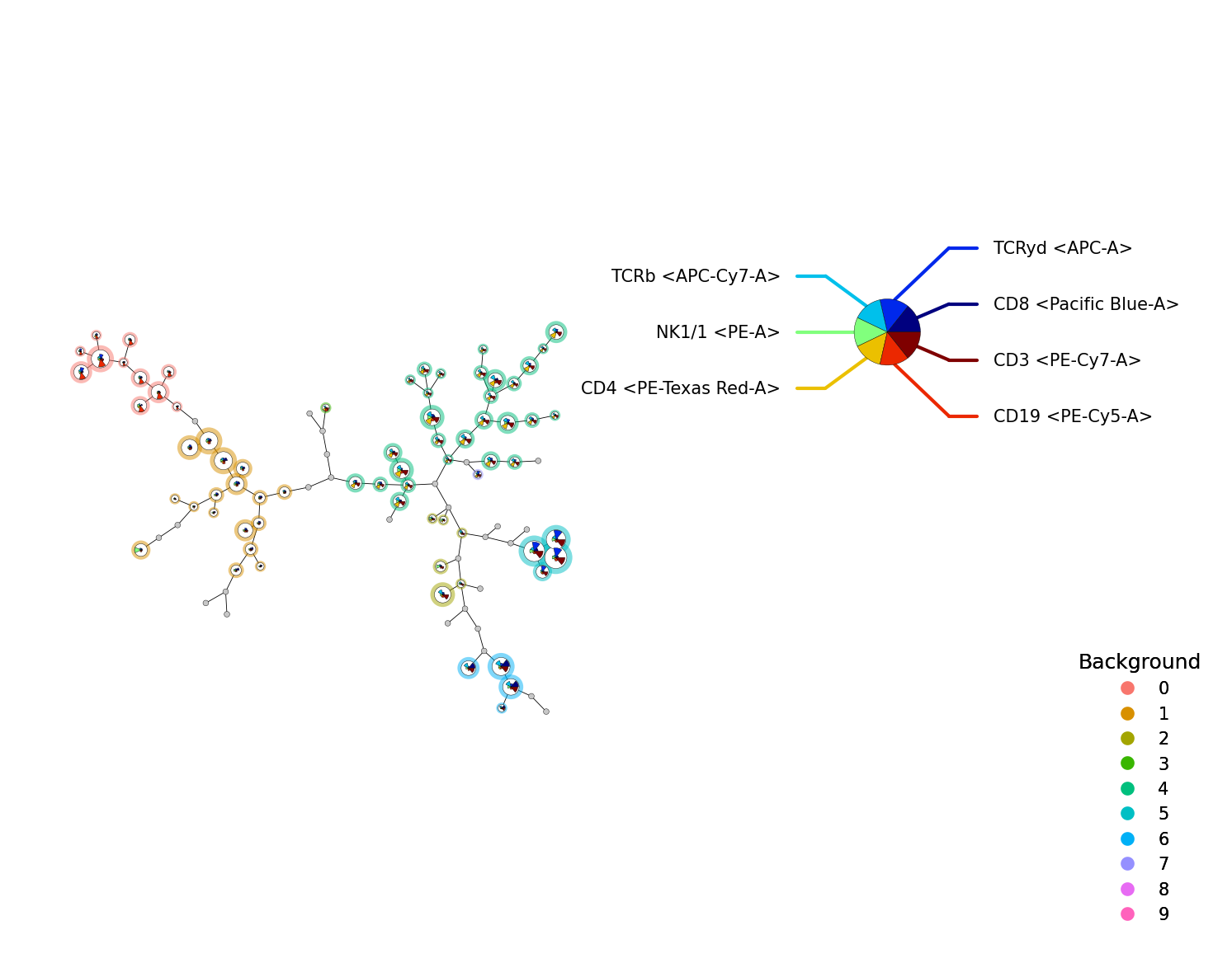
To map new data on an existing FlowSOM object, we can use the new_data() function.

fsom_new = fsom.new_data(ff_t[1:200, :])
p = fs.pl.plot_stars(fsom_new, background_values=fsom_new.get_cluster_data().obs.metaclustering)

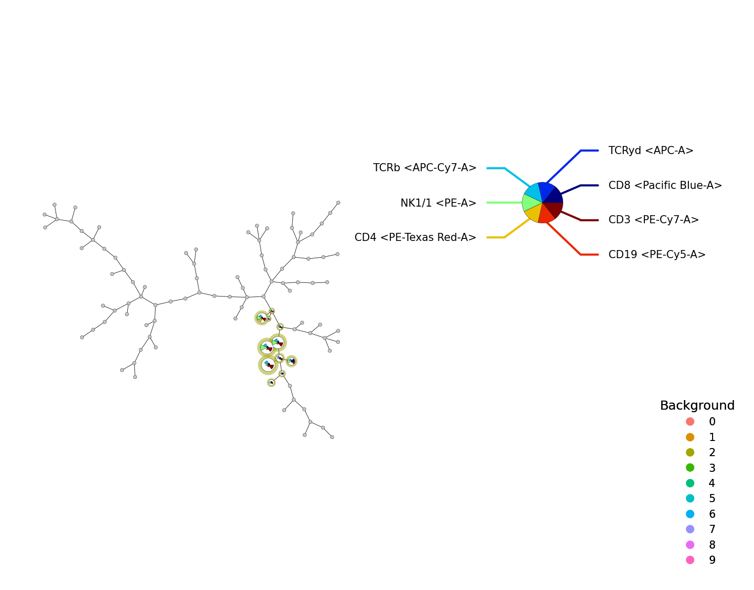
We can also take a subset of a FlowSOM object. For this we use the subset() function.

fsom_subset = fsom.subset(fsom.get_cell_data().obs["metaclustering"] == 2)
p = fs.pl.plot_stars(fsom_subset, background_values=fsom_subset.get_cluster_data().obs.metaclustering)

import session_info2

session_info2.session_info(dependencies=True)